CHAPTER
EIGHT
Case
#15 FORECAST COMBINATION WITH LINEAR AND NONLINEAR TREND
Goal: This
case examines the practice of forecast combination stressing the role of
diverse information as applied to forecasting the S&P 500 composite stock
index. Specifically, it examines:
- Forecasting
Trend using Linear Regression
- Forecasting
Nonlinear Trend with Multiple Regression
- Testing
conditions for Effective Forecast Combination
- Estimating
Optimal Weights in the Forecast Combination Process.
Problem Spreadsheet
For
this case we selected a time series characterized by no seasonality and a
non-linear trend. Since stock prices are
non-seasonal and follow exponential growth, we selected data on the S&P 500 Composite Stock Index (FSPCOM). Our purpose is to stress test the forecast
combination process by examining a case where forecast combination should fail
to produce superior results!
The
spreadsheet for this problem is C8_Case1.xls.
It contains the following data:
|
Variable |
|
|
FSPCOM |
1947Q1-1994Q4 |
|
TIME |
1947Q1-1994Q4 |
|
TIME_SQUARED |
1947Q1-1994Q4 |
The
series FSPCOM is quarterly data on the S&P 500 Composite Index. The time indices will be used to estimate a
linear and non-linear trend model.
Examining Data for
Stationarity
To examine the behavior of FSPCOM over
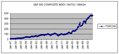
the historical period (1947Q1-1994Q4), we generated a time-series plot of the
data using Excel.

Question #1: Based upon a time-series plot, do the
quarterly data exhibit a non-linear trend?
ANSWER:
Based upon the historical plot of quarterly data shown above, the trend is
clearly non-linear as expected, since stock prices reflect compound rates of
return.
Linear Trend Regression

|
Multiple
Regression -- Result Formula |
|
|
|
||
|
|
|
|
|
|
|
|
FSPCOM
= -46.69 + ((TIME) * 1.82) |
|
|
|
||
|
|
|
|
|
|
|
|
Forecast
-- Multiple Regression Selected |
|
|
|
||
|
|
|
Forecast |
|
95% - 5% |
95% - 5% |
|
Date |
Quarterly |
Annual |
|
Upper |
Lower |
|
Jan-1995 |
304.56 |
|
|
406.76 |
202.36 |
|
Apr-1995 |
306.38 |
|
|
408.59 |
204.17 |
|
Jul-1995 |
308.20 |
|
|
410.43 |
205.97 |
|
Oct-1995 |
310.02 |
1,229.16 |
|
412.26 |
207.77 |
|
Avg |
307.29 |
1,229.16 |
|
409.51 |
205.07 |
|
Max |
310.02 |
1,229.16 |
|
412.26 |
207.77 |
|
Min |
304.56 |
1,229.16 |
|
406.76 |
202.36 |
|
Audit
Trail -- Coefficient Table (Multiple Regression Selected) |
|
|
|
|||
|
Series |
Included |
|
Standard |
|
|
Overall |
|
Description |
in Model |
Coefficient |
Error |
T-test |
Elasticity |
F-test |
|
FSPCOM |
Dependent |
-46.69 |
8.84 |
-5.28 |
|
524.56 |
|
TIME |
Yes |
1.82 |
0.08 |
22.90 |
1.36 |
|
|
Accuracy
Measures |
|
Value |
|
|
AIC |
|
|
2,123.60 |
|
BIC |
|
|
2,126.86 |
|
Mean
Absolute Percentage Error (MAPE) |
63.83% |
||
|
Sum
Squared Error (SSE) |
|
707,606.37 |
|
|
R-Square |
|
|
73.41% |
|
Adjusted
R-Square |
|
73.27% |
|
|
Root Mean
Square Error |
|
60.71 |
|
Question #2: Evaluate the quality of the linear
trend regression model.
ANSWER:
The linear model appears to fit the data well as shown by the R-squared of
.7341 and the large value of the F-statistic.
In addition, the coefficient on TIME is positive as expected, and
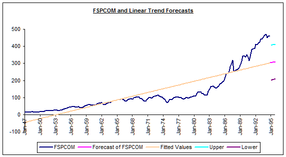
significantly different from zero at the 99% level of confidence. However, as shown by the plot of forecasts
and actual data, the model completely misses the non-linear trend apparent in
the data! Accordingly, next we
re-estimated the data using a non-linear trend regression model.
Non-Linear Trend Model
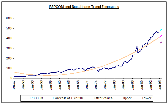
Using
FORECASTXTM, we generated forecasts of FSPCOM for 1995 along
with a holdout period for 1994 using a non-linear trend regression model. Summary results are reported below.

|
Multiple
Regression -- Result Formula |
|
|
|
||
|
|
|
|
|
|
|
|
FSPCOM
= 61.93 + ( (TIME) * -1.54 ) + ( (TIME_SQUARED) * 0.017406 ) |
|
||||
|
|
|
|
|
|
|
|
Forecast
-- Multiple Regression Selected |
|
|
|
||
|
|
|
Forecast |
|
95% - 5% |
95% - 5% |
|
Date |
Quarterly |
Annual |
|
Upper |
Lower |
|
Jan-1995 |
413.15 |
|
|
477.09 |
349.20 |
|
Apr-1995 |
418.27 |
|
|
482.28 |
354.27 |
|
Jul-1995 |
423.40 |
|
|
487.47 |
359.33 |
|
Oct-1995 |
428.53 |
1,683.35 |
|
492.67 |
364.40 |
|
Avg |
420.84 |
1,683.35 |
|
484.88 |
356.80 |
|
Max |
428.53 |
1,683.35 |
|
492.67 |
364.40 |
|
Min |
413.15 |
1,683.35 |
|
477.09 |
349.20 |
|
Audit
Trail -- Coefficient Table (Multiple Regression Selected) |
|
|
|
|||
|
Series |
Included |
|
Standard |
|
|
Overall |
|
Description |
in Model |
Coefficient |
Error |
T-test |
Elasticity |
F-test |
|
FSPCOM |
Dependent |
61.93 |
8.25 |
7.51 |
|
842.06 |
|
TIME |
Yes |
-1.54 |
0.20 |
-7.80 |
-1.15 |
|
|
TIME_SQUARED |
Yes |
0.02 |
0.00 |
17.58 |
1.67 |
|
|
Accuracy
Measures |
|
Value |
|
|
AIC |
|
|
1,937.56 |
|
BIC |
|
|
1,940.82 |
|
Mean
Absolute Percentage Error (MAPE) |
48.23% |
||
|
Sum
Squared Error (SSE) |
|
268,516.47 |
|
|
R-Square |
|
|
89.91% |
|
Adjusted
R-Square |
|
89.80% |
|
|
Chi-Square |
|
|
1.00 |
|
Cochrane-Orcutt |
|
|
0.97 |
|
Mean
Absolute Error |
|
32.90 |
|
|
Mean Error |
|
|
0.00 |
|
Mean
Square Error |
|
1,398.52 |
|
|
Normality
Error |
|
|
61.12 |
|
Root Mean
Square Error |
|
37.40 |
|
|
Standard
Deviation of Error |
|
37.49 |
|
|
Theil |
|
|
11.95 |
Question #3: Evaluate the quality of the estimated
non-linear trend model.
ANSWER: The non-linear model appears to fit the data
quite well as shown by the R-squared of .8991 and the large value of the
F-statistic. The coefficient on TIME is
negative and significantly different from zero at the 99% level of
confidence. The coefficient on
TIME_SQUARED is positive and significantly different from zero at the 99% level
of confidence, consistent with the trend being non-linear. The in-sample RMSE is 37.40, about a half of
the linear trend model!
Can These Models be Combined?
To
examine whether these two models can be combined, we estimate the following
regression:
|
Audit
Trail -- Coefficient Table (Multiple Regression Selected) |
|
|
|||
|
Series |
Included |
|
Standard |
|
Overall |
|
Description |
in Model |
Coefficient |
Error |
T-test |
F-test |
|
FSPCOM |
Dependent |
0.00 |
4.41 |
0.00 |
842.06 |
|
Linear_Forecast |
Yes |
0.00 |
0.06 |
0.00 |
|
|
Nonlinear_Forecast |
Yes |
1.00 |
0.06 |
17.58 |
|
Question #4: Based upon the estimated regression
above, can we successfully combine these two forecasting methods without
generating biased forecasts?
ANSWER: As shown by the calculated t-statistic on the
intercept term, we cannot reject the null of a zero intercept. Accordingly, we can combine the two trend
models without generating any forecast bias.
Optimal Forecast Combination
Next,
we use multiple regression to calculate optimal forecast combination weights
and forecasts for 1995.
|
Multiple
Regression -- Result Formula |
|
|
||
|
|
|
|
|
|
|
FSPCOM
= 0. + ( (Linear_Forecast) * 0. ) + ( (Nonlinear_Forecast) * 1.00 ) |
||||
|
Audit
Trail -- Coefficient Table (Multiple Regression Selected) |
|
|
|||
|
Series |
Included |
|
Standard |
|
Overall |
|
Description |
in Model |
Coefficient |
Error |
T-test |
F-test |
|
FSPCOM |
Dependent |
0.00 |
0.00 |
0.00 |
846.52 |
|
Linear_Forecast |
Yes |
0.00 |
0.06 |
0.00 |
|
|
Nonlinear_Forecast |
Yes |
1.00 |
0.06 |
17.63 |
|
Here,
the optimal weight to the linear forecast is zero! This should not be a surprise because the
information about the linear trend is already contained in the non-linear
model. In fact, any other result would
question the validity of this method of optimal combined forecasting weighting.
In-sample
accuracy results for the combined model are reported below.
|
Accuracy
Measures |
|
Value |
|
|
AIC |
|
|
1,937.56 |
|
BIC |
|
|
1,940.82 |
|
Mean
Absolute Percentage Error (MAPE) |
48.23% |
||
|
Sum
Squared Error (SSE) |
|
268,516.47 |
|
|
R-Square |
|
|
89.91% |
|
Adjusted
R-Square |
|
89.80% |
|
|
Chi-Square |
|
|
1.00 |
|
Cochrane-Orcutt |
|
|
0.97 |
|
Mean
Absolute Error |
|
32.90 |
|
|
Mean Error |
|
|
0.00 |
|
Mean
Square Error |
|
1,398.52 |
|
|
Normality
Error |
|
|
61.12 |
|
Root Mean
Square Error |
|
37.40 |
|
|
Standard
Deviation of Error |
|
37.49 |
|
|
Theil |
|
|
11.95 |
|
|
|
|
|
|
Method
Statistics |
|
Value |
|
|
Method
Selected |
|
|
Multiple Regression |
Forecasts
for 1995 are reported below.
|
Forecast
-- Multiple Regression Selected |
||
|
|
|
Forecast |
|
Date |
Quarterly |
Annual |
|
Jan-1995 |
413.12 |
|
|
Apr-1995 |
418.23 |
|
|
Jul-1995 |
423.34 |
|
|
Oct-1995 |
428.45 |
1,683.14 |
|
Avg |
420.78 |
1,683.14 |
|
Max |
428.45 |
1,683.14 |
|
Min |
413.12 |
1,683.14 |
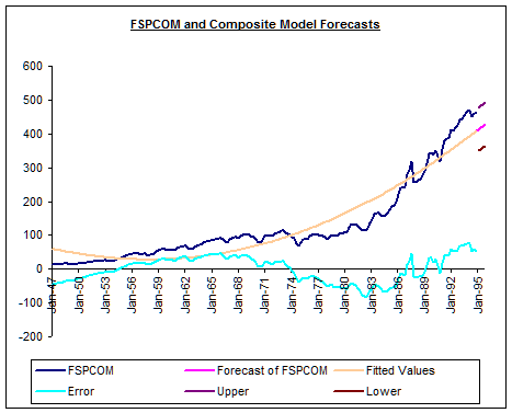
A
plot of FSPCOM and combined forecasts is shown below.

Question #5: Based upon the results above, do the
combined forecasts outperform the other models? Explain.
ANSWER:
As shown above, the weight given to the linear model is essentially zero. Accordingly, there is no gain to combining
the linear and non-linear trend models.
Indeed,
the combined forecasts and statistics are exactly the same as those of the
non-linear trend model. The point: For forecast combination to work you must
employ differing information in the methods you combine!
Student Practice Question
Question #1: What improvement do you expect in
forecast accuracy if we include the time index raised to the third power, i.e.,
allow a S-shaped trend? Using FORECASTXTM,
test your theory on the data of this case study. Explain!